Author: joshua.chelakkattuparambil

Overall I must say, it was quite a journey. Navigating my way through the various errors and setbacks I faced was truly soul crushing at times. I often didn’t know how to proceed and felt completely frozen and helpless. However, I always received assistance from my mentor, Mr. Sontacchi, who motivated me to push through till the end. He has guided me through many obstacles I faced and helped me re-establish interest in the project when I thought I couldn’t make it happen. I would like to personally thank him for all the effort he has put in and the support he’s given me throughout this semester.

One thing I wish I had was more time to focus specifically on this project. There were various scenarios where I was caught between multiple deadlines, which restricted me from focusing on what I wanted to achieve. It was frustrating as I wanted to progress and move forward with the work but was held back due to the workload from the other courses. Balancing the time for this research project alongside the other project felt difficult. I felt this project could have been even more expansive if I had more time to contribute to it. 

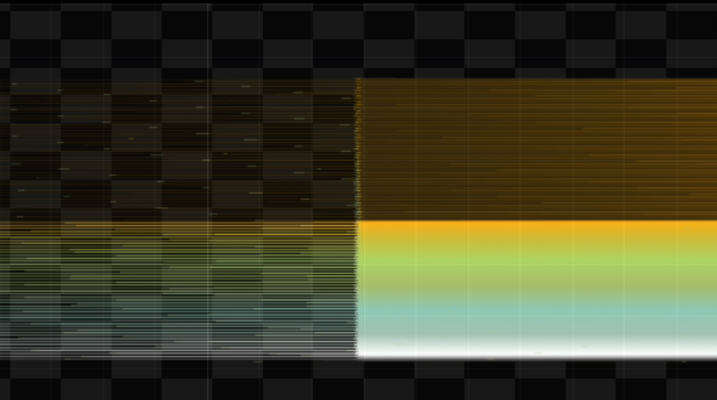
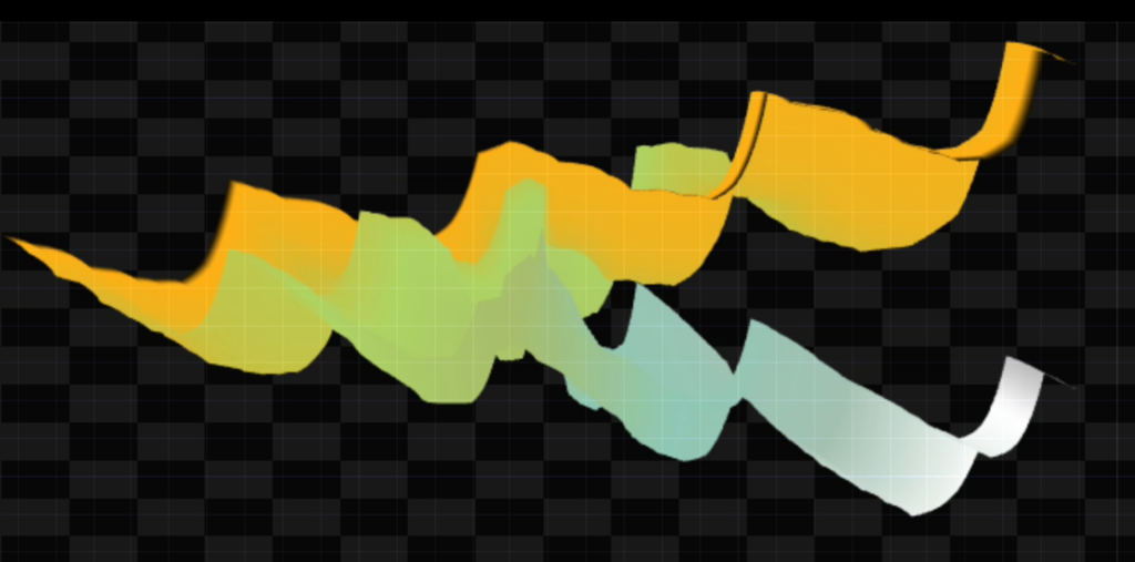
One of the things that I had to change was the model of the waveform for the visualizer. I initially intended to work on a 3D waveform, with more particle clouds and points, but it turned out to be more complicated than I had initially expected. Through my mentor’s guidance, I built the existing model, which varies in pitch based on its position on the y-axis. I really like the current model, but would like to rework it and build an alternative for the final installation. 

Additionally, I wish to integrate the pitch to colour mapping in some form. I am planning to map harmonics and timbre to the properties of the newly designed visualizer. I also need to implement a surround sound system for the audio response to recreate an immersive environment, as well as offer additional control parameters such as playback loudness, directional panning and wet/dry mix of the output. There is a lot of testing that needs to be done to ensure we don’t suffer from latency issues.

In the end I am happy with the output and super glad to have a functioning prototype to present. That being said, I still believe there is a lot of work to be done in the upcoming semester for me to completely realize the installation that I had envisioned. I am looking forward to continuing work on this research project.

My prototype for this semester is finally complete. After much trial and error, I was able to build a visualizer that functions as per the user’s input and is represented in a model that is easily understandable to the user. The waveform morphs and reacts based on the user input and doesn’t break or alter its core geometry in the process, finally maintaining a smooth and fluid visual experience. There are still a few additional tweaks that can be done, but it’s somewhat functional at the moment, which means that I have met my primary goals for this semester.

Some additions include the audio feedback response, which acts as a monitor based on chords to determine the pitch accuracy of the user. This was done using the quality parameter in the sigmund object, a very useful tool for pitch tracking. The signal runs through a relational operator (>) and when the signal fulfills the condition (greater than 90%), the patch plays back a chord for the user from an oscillator based on their pitch quality. If the user is perfectly in pitch, it will play a pleasant major chord, while a slightly off-pitch input would trigger a more dissonant minor chord, providing immediate auditory feedback without the user needing to look at a screen.

Another addition is the waveform, which now features a visual activation response where the visualiser remains inactive or dark when there is little to no input signal. The colour in the waveform reappears when the user is speaking, and this is a vital visual feature to indicate that the signal is being successfully received from the user. By fading to dark during silence, the interface reduces visual fatigue and makes the interactive moments feel much more dynamic. This addition was done using the data from the quality argument in the sigmund object, which was mapped to a Logic CHOP in TouchDesigner to trigger the visual state changes seamlessly.

I also considered adding a few advanced audio analysis tools from a Python library to give users more speech information. What I had imagined was an algorithm which collects a live data feed and predicts the different groups of consonants present in the speech (fricatives, affricates, plosives, etc). You would see numbers fluctuating on screen showing the variations in frequency as well as the tonal quality.  Unfortunately, I won’t have enough time to implement this into the prototype, and it would be considered as a feature to be added in the future.

In the final blog, I will share my overall experience building the prototype, reflect on the challenges, and give insights on what to look forward to in the upcoming semester.

Last month, the sound designers and exhibition designers of FH Joanneum jointly participated in an excursion to the Ars Electronica Center in Linz. The center is a museum that focuses on new media art and is most renowned for its annual festival, the Ars Electronica Festival, which critics have praised as a pivotal exhibition in the digital arts. It is widely considered one of the best known creative arts festivals in Austria. Over the years, the people behind the center have been praised for their unique integration of technology into the creative field. They also have a dedicated inhouse research facility called the Futurelab, which focuses on modern technological advancements, particularly artificial intelligence. 

There were a lot of engaging exhibits. Some memorable ones included the fascinating “tardigrade” under a microscope, as it made its way through its tiny surroundings. These remarkable creatures are incredibly resilient, capable of withstanding extreme temperatures and are known to be some of the only organisms able to survive in outer space. Another interesting part of the excursion was the Deep Space 8K experience, which drew us into a world of 3D visuals. We heard various soundscapes, ranging from the planets of our solar system to our oceans, and even the unique art of yodelling.

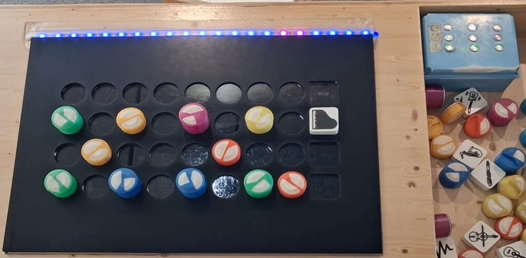
The exhibit I would like to speak about in detail is the simple sequencer, which was located in the Kids Research Lab on the first floor of the building. I really enjoyed the sequencer and felt like a kid again while playing around with it for some time. It was a really nice setup, especially for children who are curious about music and sound in general. It was a simple concept, but one that was very much fun to use due to the various patterns you could recreate.

The sequencer was off by default, so you had to place blocks (or tiles) representing a particular instrument onto the vacant slots to produce sounds. On the left hand side of the instrument block was the fill pattern, consisting of 8 distinct beats that the user could customize to recreate a unique rhythm. There was an LED strip on the top edge of the sequencer, which indicated the beat being played at the time. The beat blocks came in different colours and sizes. Some were taller than the others and had unique shapes on the top facing size. However, I was not able to decipher exactly what these could have stood for. This may have possibly been a measure used for quarter or half notes, but I am not entirely sure. The instrument blocks included an acoustic guitar, a piano, an electric bass and even a saxophone.

The sequencer could only accommodate 4 instruments at a time as there were only 4 slots available. Apart from this, there was also a small blue box on the right side of the sequencer with buttons featuring images of snares, cymbals and kick drums. I do not recall if these sounds played in sync with the sequencer but pressing them did produce the sounds of the instruments I just described.

Overall, I really enjoyed the visit and gained valuable insights from the unique exhibits. From the way they were presented to the overall setup of the installations, it was a good trip to explore and brainstorm ideas for our own installations at Klanglicht later this year. 

Building the visualizer was the most challenging part of the project so far. I ran into a lot of trouble fixing the waveform as it kept changing drastically through each iteration. In this post, I will give a breakdown of the workflow and briefly discuss the multiple errors I faced along the way.

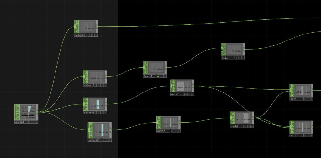
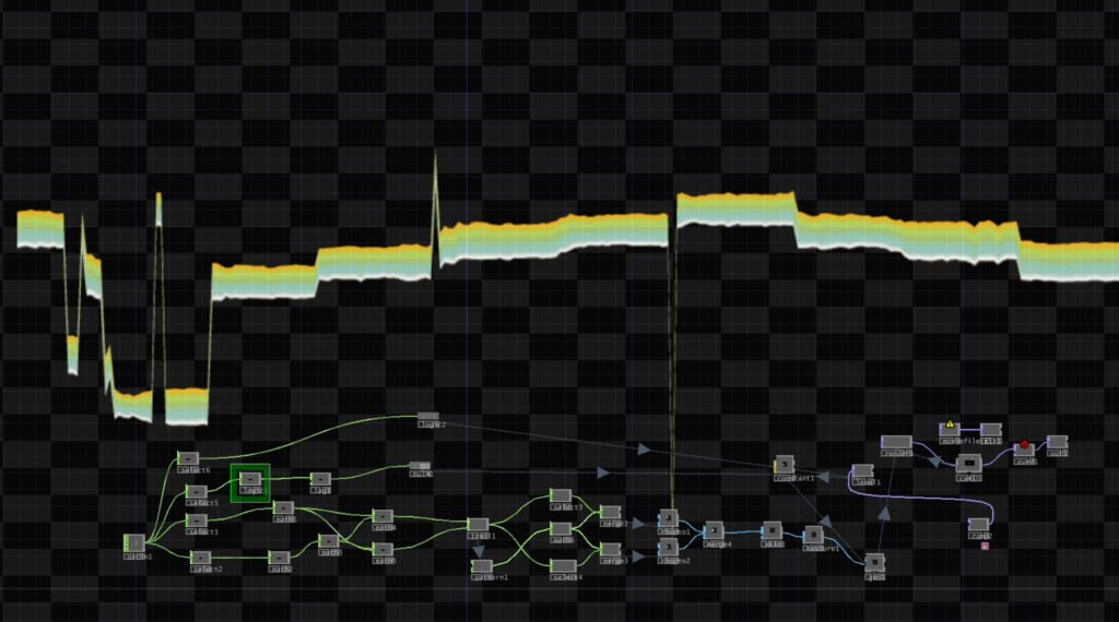
I built the ribbon based visual system using multiple elements as I mentioned in the last blog, utilizing various combinations of multiple CHOPs (channel operators), TOPs (texture operators) and SOPs (surface operators) to get the output. I initially used an OSC In CHOP to collect the data on pitch and loudness. These data streams were then separated using a select CHOP and sent to a math CHOP to define the parameter ranges. This was a crucial step, as defining these ranges significantly altered the visualizer’s behaviour. I finally settled on a ‘from range’ of 40 to 100 and a ‘to range’ of 0 to 4 for the pitch. The loudness, meanwhile, has a ‘from range’ of 25 to 100 and the ‘to range’ of 0 to 2.

I had to create more math CHOPs to carry out more calculations. I split the loudness in half and combined it with the pitch values through the operation of addition and subtraction. This was done to define the upper and lower limit of the waveform, which were called ‘ty_top’ and ‘ty_bottom’ respectively. After this series of math CHOPs I had to place a Trail CHOP to capture the history of the data, recreating the continuous stream of data at the given timeframe. This was followed by the pattern CHOP, which served as data for the x-axis. The pattern chop was then sent through a math chop and merged with the individual channels (ty_top and ty_bottom). Once this was done, we converted the CHOP to SOP for adding surfaces and textures. Finally, the SOP was placed into a Geometry COMP then a camera TOP and a render TOP were added to the end of the signal chain to generate the final visual output.

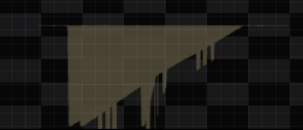
This basically makes up the entire visual build, but there were a lot of errors that occurred along the way. The first reoccuring issue was the appearance of a static line despite signals being received through OSC. Another visual bug was these sharp, triangular shapes that kept being pushed from the center, it looked very confusing. I also had multiple scenarios where the signal did not rise along the y-axis with the variation in pitch. And at times, we also had signals literally break in two halfway through the visualizer. It became so bad I started a new visual project in Processing, as it felt more likely to give me the output I was expecting.

In the end, I am trying to achieve a functional model with a few additional features that help the visualizer feel more interactive and complete.

In the last blog, I discussed the functioning and features of the audio pipeline, which was built using plugdata. We were able to collect pitch and loudness data from our audio stream and were attempting to send it to TouchDesigner via OSC. However, the connection was not successful. I had to redo the patch and will share my insights and methodology on fixing the issues.

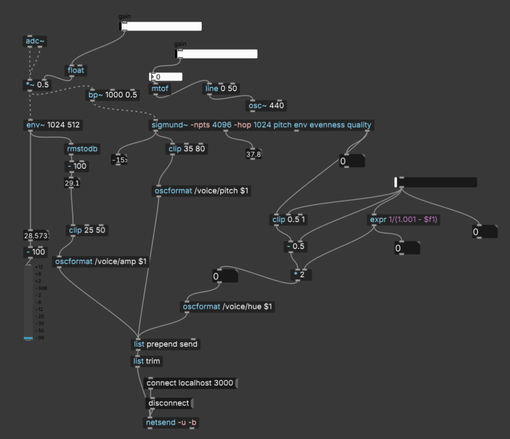
I had to repackage the data streams into an [oscformat] object and then prepend them into a list before moving on to the next step, which was to replace the [oscsend] object I had previously used with a [netsend] object containing the arguments ‘-u’ and ‘-b’. This sends data through the UDP protocol. It was configured to send messages to localhost on the port I set at 3000. 

In TouchDesigner, I used the ‘OSC In CHOP’ to collect the information sent from plugdata. I had a small monitor indicating the variations in values inside the CHOP, this meant that the data connection was successful. I was now ready to build the audio reactive visualizer. I wanted to see how the OSC data affected the visual output. So, I tried testing it out with a project I found through the Youtube channel supermarket sallad. It was a spherical visualizer which simulated various particles and noise. It was a visually appealing piece, I was able to play around with the lighting along with particles and found it really interesting. I wanted to implement a similar visual model with particle clouds for my project but later decided to go with an alternate approach.

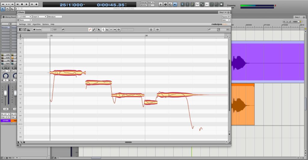
My initial concept was to build a 3D waveform model for the visualizer, but it was proving to be quite difficult. After consulting with my mentor, he suggested that I work on a simpler model and if needed modify it later on. I was now trying to think and come up with ideas for new visualizer styles which can also be easily understood by a user. So, I kept searching and eventually got curious with the waveform structures found in pitch shifting plugins like Melodyne. It seemed like an interesting model as you could tell the variation in pitch based on different positions along the y-axis. This also made me move away from mapping pitches to colour (Camelot wheel) as I had described earlier.

I would still have to consider a couple of things to see if this model works for me. What kind of elements (CHOPs, SOPs, TOPs) would I require to build this model and how accurately can I display the concept I had initially planned? Some of these will be answered in my next blog. Until then!

The first step to build my working prototype was to start with the Pure Data patch. This is an integral part of the project as all the live data is being collected and parsed through these connections. I used an alternate version of Pure data called plugdata. I found it more convenient to work with as it has a much more modern UI, helping users (especially me) navigate the software easily.

So, my intention behind this patch was to build a system to collect live audio signals, retrieve information about pitch and loudness of these signals, and store them in lists which can be sent to OSC for TouchDesigner to collect and interpret. The audio signal is captured using an [adc~] object which is then amplified using a [*~] object which is connected to a horizontal slider to ensure input gain can be controlled by the user. This is one of our most important control parameters. The patch then analyzes the audio stream and splits it into the two properties that I mentioned earlier, pitch and loudness.

In order to obtain loudness information, we had to use the RMS value which can be computed using the [env~] object. I wanted to use decibels for the project, as it is the most commonly used measurement for playback systems. In order to achieve this, I used the [rmstodb] object. To test if the signal was functioning as expected, a VU meter was connected to monitor the signal. This was then connected to an oscsend for the data to be transmitted.

As for the pitch, it was slightly more complex. I had to use the [sigmund~] object with the arguments ‘-pitch’ and ‘-peaks’ to obtain the values. I was not familiar with this object and it took me some time to understand the working behind it. It continuously analyzes the waveform to track fundamental frequency. The frequency value is then passed through an [ftom] object which converts frequency into MIDI objects. This helps to work with musical notes that are more familiar. It is also much easier to map to visual parameters. These MIDI values are also sent through OSC for TouchDesigner to collect and process.

My next step is to test the OSC data and ensure it is being received correctly by TouchDesigner. Should be simpler considering the data being transferred locally. Localhost should suffice for this and netsend might also do the trick. My findings will be revealed in the next blog. Stay tuned!

One thing I had to take into consideration while building the prototype was defining the parameters we were going to use for the project. Obviously, being an audio reactive visualizer, the two most relevant (and important) parameters to map would be the loudness and pitch of the input signal produced by the user. These quantities will be mapped to affect the position, shape and texture of the visualizer. Sounds simple enough. So, how exactly will this be done? What is affecting what here? To answer that question, we need to delve a little bit into colour theory based on the Camelot wheel.

My idea for mapping the user’s pitch is to base it on the Camelot wheel, a visual tool often used by DJs to help with harmonic mixing. It is based on the principle of the ‘Circle of Fifths’, which maps out all 12 musical keys in a visual clock format, highlighting the different relations between them. The Camelot wheel turns this into a shorthand guide by using numbers (1-12) denoting each fundamental musical key and letters (A & B) representing the scale types. ‘A’ indicates minor keys while ‘B’ highlights major keys. It is usually visualized as a rainbow wheel, but it does not really hold any true correlation between the colours and the notes. I would like to build a type of cross modal correspondence and relate colours to notes, indicating variations in pitch through colour differences.

The loudness parameter was a more intuitive choice. I based this on the waveforms we see today, a very obvious correlation to represent loudness levels. The louder the sound, the higher the peak of the waveform. It will be interesting to see if we could recreate a highly dynamic waveform based on the user’s voice. This also serves as a commentary (no pun intended) on the loudness wars, which we still see today. Most tracks produced today are so heavily compressed to the point that they appear as continuous peak waveforms, losing the unique dynamic quality of each particular instrument and audiotrack.

Two other things we need to consider are the sensitivity of the visualizer’s response to the input and how it can be fine tuned to get the best possible results. We also need to ensure the dataset is normalized such that it is suitable for our visualizer to interpret. Because huge variations in range can massively alter and shift the output. The biggest hurdle will be finding the exact range or measure to ensure the visualizer functions exactly as we need it to.

The human voice is such a fascinating tool, yet so complex. My project is heavily dependent on input signals based on human speech and so I considered doing some dedicated research on it. I was quite astonished by the results and was surprised to discover this world of phonetics and linguistics, which were so new to me.

I wanted to dive deeper and understand the ways the sounds in human speech differ and see just how varied they are. This brought me back to one of the assignments I did last semester for the Digital Signal Processing course. We were asked to record different vowels and analyze the distinctions between them. Formants were identified as the primary acoustic cues for vowel identification. The differences between the first two formant frequencies (F1 and F2) helped us distinguish each vowel. 

For instance, in our exercise the vowel “U” only had a difference of 500 Hz, while a vowel like “E” had a difference of over 1600 Hz. The vocal tract acts as a filter, by altering the position of the tongue, jaw, and lips the speaker changes the shape of this resonating tube. This physical manipulation amplifies specific frequency bands (formants) while dampening others.

Apart from this, we also have consonants which possess their own unique characteristics. In English phonology, consonants can be split into 6 different categories based on their articulation. These include plosives, fricatives, affricates, nasals, approximants and laterals. These sounds are produced based on variations in airflow between the vocal tract and lips. Additionally, linguists have classified these consonants into 2 categories based on voicing: voiced (where the vocal cords vibrate when the sound is made) and voiceless (where the vocal cords do not vibrate, and the sound is shaped purely by breath).

While figuring out ways to test out these consonants with my prototype, I realized it would be cool to experiment with modern day beatboxing. I was inspired to do this while watching a WIRED video about the different levels of beatboxing. Popularized by the African American communities in the US during the mid 80s, it grew into a huge sensation and remains a staple in pop culture today. It would be a really cool way to experiment and analyze speech, as these artists use fricatives and plosives to recreate the rhythms similar to a drumkit. I am curious to see how this will turn out.

This also made me realize that I could add some sort of live audio detection tool for speech analysis. I am planning to search for a few Python libraries I could use to achieve this. This could be a very interesting add on to the project and would validate important information about the phonetic structure of the speech, providing valuable insights for singers, voice actors and other professionals working with the human voice.

In this first blog for the Einzelprojekt, I plan on discusssing the various fields of study I will delve into for my research project and how they associate with the courses I am currently attending. My focus for this semester is to build a functional prototype, test it and ensure that it runs exactly as I expect it to.

Before we dive deep into it, I would like to give a short recap of my project. The primary idea is to build an interactive visualizer which responds to real time audio data. It identifies vocal characteristics and maps auditory features like pitch and loudness onto visual dimensions such as size, shape, colour and texture.This model will be further developed and used to build an immersive installation where users can modify and create unique audiovisual pieces using the provided parameters.

Speaking of parameters, I recently had a detailed class explaining parameter mapping, a commonly used method for sonification of data. What I found fascinating is the step by step process of data structuring to generate a definitive output, ensuring the results align with research hypotheses. It involves defining data dimensions and mapping them to sound parameters such as pitch and loudness (both of which I will explore in my project). Finding the right dataset, parsing it and normalizing it within ranges suitable for the project are also crucial steps. This requires a lot of iterations and testing, which I’m sure I will have to do in my project as well.

Another interesting class I am currently taking part in is the ambisonics and surroundsound lectures held at the CUBE. We went over the various orders of ambisonics and listened to the differences in each format. I will be working on a soundscape for this course at the end of this semester, which will help me understand the spatial positioning and panning within an ambisonic environment. I won’t be focusing heavily on spatialisation for my project this semester, either way it is incredibly valuable to my research and will provide me with ideas for integrating this setup into my installation next semester.

I am primarily focused on building this prototype using plugdata and TouchDesigner. I am currently working on projects in both software environments for the Musikmaschine installation and the sound & vision exhibition, respectively. I am trying to grasp as much information as I can so I can transfer those same methodologies to this project.

I am really excited to see how this project unfolds. There are bound to be hurdles along the way, but I am positive I will reach my goal by the end of this semester and successfully complete the entire installation by the end of the next.

The previous blog focused primarily on workshops rooted in neuroscientific research. The following three delve into digital signal processing, visual generation from audio and dynamic spatialisation. Each of these highlights features I am planning to integrate into my personal project.

Moving with time

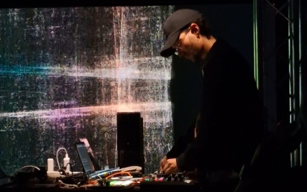
Moving with Time is an immersive audiovisual performance exploring the evolving relationship between sound, image, and culture through real-time interaction. Amongst all the projects I have seen and been a part of during the entirety of the workshop, this particular performance had the closest semblance to my research project.

Some of the common processes this project shares with the research project include real-time digital signal processing, transforming sound and modifying it in real time. They had used granular and concatenative synthesis in Max/MSP to achieve this. I am still unsure whether to include this in my project, but I would definitely implement an interactive feature for users to stay engaged with the installation. Another common element present in both projects is real-time visual generation, made using TouchDesigner. 

Speaking about the performance, I personally really enjoyed the fusion of music styles from the traditional Persian Setar to the warm textures of the ARP Odyssey and the Monotribe, it progressively builds and resolves eloquently.

Generative Music from the Quantum World

I could have never  imagined using quantum mechanics to make music until Jean-Claude Heudin had talked about it. In this fascinating presentation, we were introduced to ANGELIA, a hybrid generative AI developed to enhance the creativity of the artist for composing, and to augment performative capabilities.

Heudin briefly explained some fundamental concepts of quantum mechanics like superposition, entanglement and measurement (or collapse). He also mentioned how qubits that exist in superposition states, can be subjected to incompatible measurements, and even be entangled with other qubits.

We were also introduced to Qunotes, which are like qubits but with musical notes instead of binary information. The quantum state of a qunote is represented by a linear superposition of a defined number of pitch values. It’s only when the piece of quantum music is played that a qunote collapses into a defined state. Each time the same qunote plays, a different note is obtained depending on the probability amplitudes. This results in many possible interpretations of the same score. Therefore, the composing is done with probability amplitudes instead of fixed notes.

Dynamic Spatial Mixing for Multi-Channel Audio

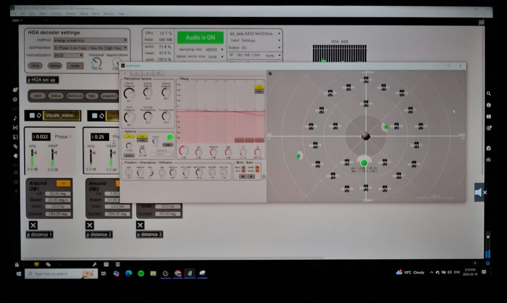
I was drawn to this project due to our course this semester (Surround Sound and spatialization). I also wanted to know more about spatial rendering and how to implement this in a mixing environment.  This live demo introduces a system for dynamic spatialization and mixing in multi-channel environments using Max/MSP and IRCAM’s SPAT library. The framework combines adaptive spatial rendering with dynamic mixing to create an evolving, responsive sonic field.

It is a unique approach to spatialisation as they combined higher order ambisonics and VBAP to achieve a unified spatial rendering system.The term they used to describe this process is ‘sidechaining’, similar to the one we use in mixing, as audio objects dynamically influence one another and interact with static beds, generating shifting amplitude and frequency relationships and establishing priority-based behaviour between moving and static spatial elements. A parallel binaural rendering was implemented into the system for headphone users as well.

Overall, I found all the sessions at the IRCAM Forum very insightful. There was a diverse mix of topics and workshops hosted by artists, performers, researchers, engineers and so on. I was able to gather a lot of interesting ideas and got introduced to some really cool concepts, some of which I would attempt to apply to my research project.